It's Convex if You Tilt Your Head a Bit

In this post, I discuss some techniques to deal with fractional objective functions which are not convex as given but can still be tackled using the tools of convex optimization. We'll explore these techniques using a specific example: choosing the portfolio with the maximum Sharpe ratio.

Markowitz portfolio construction

First some background on portfolio construction. Consider choosing a portfolio of (long-only) positions $x$ which have estimated returns $\mu$ and covariance $\Sigma$ . Often we aim to construct a portfolio that balances risk and return. A standard technique is Markowitz mean-variance portfolio optimization (see [BV04^[1] 4.4]), which solves the convex optimization problem

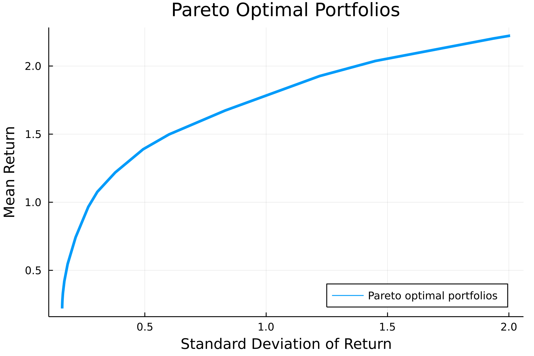
\begin{aligned} &\text{maximize} &&\mu^Tx - \gamma x^T\Sigma x \\ &\text{subject to} &&\mathbf{1}^Tx = 1 \\ &&&x \geq 0, \end{aligned}

where $\gamma$ is a parameter that controls the tradeoff between risk and return. We can easily plot this tradeoff curve (for simulated data) using the convex optimization domain specific language (DSL) Convex.jl and the solver Hypatia.jl.

using LinearAlgebra, Random, SparseArrays, Printf
using Convex, Hypatia
using Plots

# Create data
Random.seed!(0)
k, n = 5, 20
F = sprandn(n, k, 0.5)
D = Diagonal(rand(n) * sqrt(k))
Σ = Matrix(D + F*F')
μ = randn(n)

# Vary γ to plot tradeoff curve
N = 30
rets = zeros(N)
σs = zeros(N)
γs = 10 .^ range(-4, 3, N)

# Solve Markowitz problem with each γ
x = Variable(n)
for (ind, γ) in enumerate(γs)
    markowitz = maximize(μ'*x - γ*quadform(x, Σ), sum(x) == 1, x >= 0)
    solve!(markowitz, () -> Hypatia.Optimizer(); silent_solver=true)
    rets[ind] = dot(μ, x.value)
    σs[ind] = sqrt(dot(x.value, Σ, x.value))
end

plt = plot(
    σs, 
    rets,
    lw=3,
    xlabel="Standard Deviation of Return",
    ylabel="Mean Return",
    title="Pareto Optimal Portfolios",
    label="Pareto optimal portfolios",
    dpi=300,
    legend=:bottomright
)

Maximizing the Sharpe ratio

A parameter-free alternative to the formulation above is to maximize the Sharpe ratio of a long-only portfolio:

\begin{aligned} &\text{maximize} &&\frac{\mu^Tx}{\sqrt{x^T\Sigma x}} \\ &\text{subject to} &&\mathbf{1}^Tx = 1 \\ &&&x \geq 0. \end{aligned}

Intuitively, we seek to maximize the return we get per unit of risk (standard deviation). We note that the objective function

f(x) = \frac{\mu^Tx}{\sqrt{x^T\Sigma x}}

is nonconvex, so it cannot be directly tackled by a convex optimization solver. However, there are standard techniques to deal with these fractional programming problems.

Taking advantage of homogeneity

We can take advantage of the fact that the objective $f$ is 1-homogenous, i.e., $f(\alpha x) = \alpha f(x)$ for $\alpha \in \mathbb{R}_{++}$ , to transform the problem into a more friendly form. The general idea is to introduce some scaling factor $\alpha$ such that either the numerator or denominator is fixed to be $1$ . We'll work with a new variable $y = \alpha x$ and reformulate the optimization problem as

\begin{aligned} &\text{maximize} &&\frac{1}{\sqrt{y^T\Sigma y}} \\ &\text{subject to} &&\mu^Ty = 1 \\ &&&y \geq 0. \end{aligned}

Note that we no longer need the normalization constraint; we simply let

\alpha = \mathbf{1}^Ty,

so that $\mathbf{1}^Tx = \mathbf{1}^T\left(y / \alpha\right) = 1$ . The reformulated problem is equivalent to a convex quadratic program:

\begin{aligned} &\text{minimize} &&y^T\Sigma y \\ &\text{subject to} &&\mu^Ty = 1 \\ & &&y \geq 0. \end{aligned}

After solving this for $y^\star$ , we can recover the solution to the initial problem

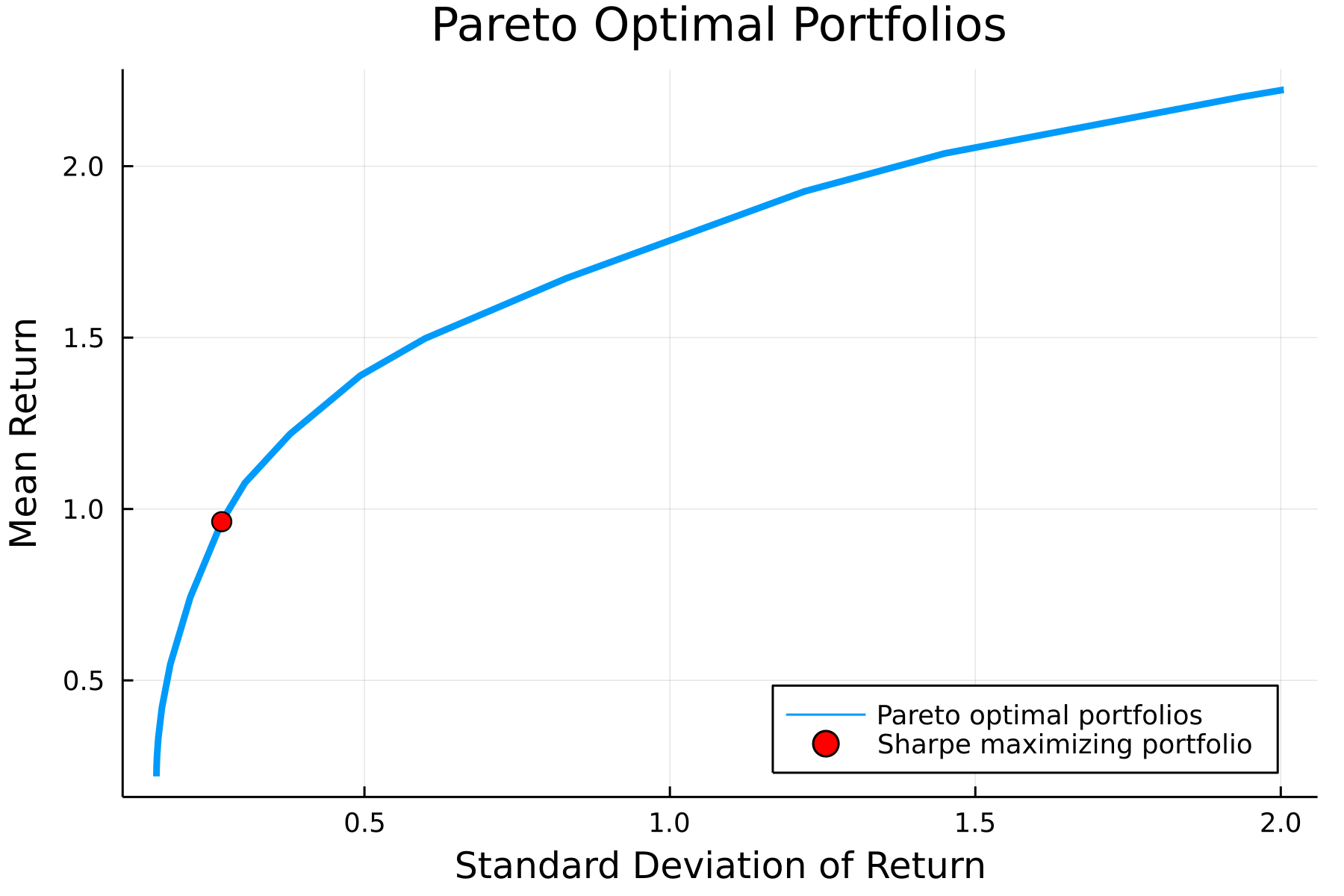
x^\star = \alpha y^\star = \frac{y^\star}{\mathbf{1}^Ty^\star},

which satisfies our constraints by construction. We can the maximum Sharpe ratio portfolio in a few lines of code:

# Construct Sharpe ratio optimization problem
y = Variable(n)
sharpe1 = minimize(quadform(y, Σ), μ'*y == 1, y >= 0)
solve!(sharpe1, () -> Hypatia.Optimizer(); silent_solver=true)

# Recover portfolio
xs = y.value ./ sum(y.value)
ret = dot(μ, xs)
σ = sqrt(dot(xs, Σ, xs))
plot!(plt,
    [σ],
    [ret],
    label="Sharpe maximizing portfolio",
    markershape=:circle,
    markercolor=:red,
    markersize=5,
    seriestype=:scatter
)

A more general approach

More generally, we consider the concave-convex fractional programming problem

\begin{aligned} &\text{maximize} &&\frac{f(x)}{g(x)} \\ &\text{subject to} && x \in S &\end{aligned}

where $f$ is nonnegative concave, $g$ is positive convex, and $S$ is a compact convex set. To transform this problem into something tractable, we introduce the new variables

y = \frac{x}{g(x)}, \qquad t = \frac{1}{g(x)}.

If $f(x) \geq 0$ on $S$ , then the optimization problem

\begin{aligned} &\text{maximize} && t\cdot f(y/t) \\ &\text{subject to} && y/t \in S \\ & && t\cdot g(y/t) \leq 1 \\ & && t > 0 \end{aligned}

is equivalent to (8) [Schaible74[2]]. (Note the relaxation of the inequality.) We note that the perspective transforms of $f$ and $g$ preserve concavity and convexity respectively [BV04^[1] 3.2.6]. Furthermore, the image and inverse images of $S$ under the perspective transform are convex [BV04^[1] 2.3.3], so

S' = \{(y,t)\mid y/t \in S, \; t > 0\}

is a convex set. Thus, the problem above is a convex optimization problem. We recently used the same idea for an optimization problem that appears in photonics.

Applying this to the Sharpe ratio problem:

It is reasonable to assume that $\mu^Tx \geq 0$ on $x \geq 0$ , as we can usually hold a portion of our assets in cash ( $\mu_n = 1$ ). Therefore, including negative returns is silly (something something inflation, I know, but this isn't a finance post). We let $f(x) = \mu^Tx$ , which is concave, and $g(x) = \sqrt{x^T\Sigma x} = \|x\|_\Sigma$ , which is convex. Applying the methods above and simplifying, we get the convex optimization problem

\begin{aligned} &\text{maximize} && \mu^Ty \\ &\text{subject to} && y \geq 0 \\ & && \mathbf{1}^Ty > 0\\ & && \|y\|_\Sigma \leq 1 \\ %& t > 0.%%%% \end{aligned}

We can solve this and verify it gives the same solution as our approach using homogeneity.

# Sharpe ratio optimization: 2nd approach
y_2 = Variable(n)
sharpe2 = maximize(μ'*y_2, quadform(y_2, Σ) <= 1, y_2 >= 0)
solve!(sharpe2, () -> Hypatia.Optimizer(); silent_solver=true)

# Recover portfolio
x_sharpe_2 = y_2.value ./ sum(y_2.value)
ret2 = dot(μ, x_sharpe_2)
σ2 = sqrt(dot(x_sharpe_2, Σ, x_sharpe_2))

# Compare approaches
rel_error_ret = abs(ret - ret2) / min(ret, ret2)
rel_error_σ = abs(σ - σ2) / min(σ, σ2)
println(
    "Relative error between approaches:" *
    "\n - mean return: $(@sprintf("%.2g", rel_error_ret))" * 
    "\n - standard deviation: $(@sprintf("%.2g", rel_error_σ))"
)

Relative error between approaches:
 - mean return: 1.2e-07
 - standard deviation: 1.1e-07

Concluding thoughts

In general, a lot of problems that don't look convex at first glance (or cannot be readily input into a solver) are tractable after a simple transformation. Disciplined Convex Programming (DCP) modeling tools like Convex.jl and CVXPY (which has extended DCP to classes of problems like log-log convex programs) help with a lot of these transformations, but many still require a manual approach.

Perhaps future optimization DSL's will be able to recognize a much larger class of convex problems automatically and apply the needed transformations. I'm pretty interested in this topic. If you are too, don't hesitate to reach out!

Thank you to Guillermo Angeris for helpful comments on a draft of this post!

References

^[1] Boyd, S., Boyd, S. P., & Vandenberghe, L. (2004). Convex optimization. Cambridge university press.

^[2] Schaible, S. (1974). Parameter-free convex equivalent and dual programs of fractional programming problems. Zeitschrift für Operations Research, 18(5), 187-196.