The Convex Boundary of Nonconvexity

Nonconvexity remains an optimization bogeyman. We solve nonconvex mixed integer problems (NP-complete!) reliably at scale for many applications. On the other hand, convex semidefinite programs––for which we know polynomial-time algorithms–-remain challenging to solve in practice.^[1] The boundary between optimization problems we can solve and those we cannot is subtle.

So when is nonconvexity relatively benign? Some nonconvex problems can be transformed into easily-solved convex ones.^[2] However, others can be reasonably tackled directly. In this post, I'll discuss one class of these problems: when you're dealing with the sum of many variables constrained to nonconvex sets. The Shapley–Folkman lemma tells us how closely this class of nonconvex problems resemble convex ones.

The Shapley–Folkman lemma

The Shapley-Folkman lemma essentially states that if you (Minkowski) sum^[3] enough nonconvex sets together, the result looks closer and closer to the convex hull. I think of this lemma as a "central limit theorem" of convex geometry. The sets are might be poorly behaved on their own, but their sum is much nicer!

The figure below of the 1/2-norm ball, repeatedly summed with itself, gives the idea:

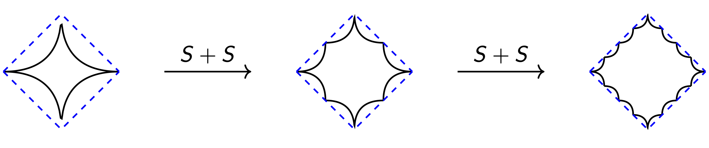
As the number of sets gets large, the sum becomes closer and closer to its convex hull. More precisely, take sets $S_1, \dots, S_m \subseteq \mathbf{R}^{n}$ and let $S$ be the convex hull of their sum:

S = \mathbf{conv}\left(\textstyle \sum_{i=1}^n S_i\right) = \sum_{i=1}^n \mathbf{conv}(S_i).

Then, for any vector $y \in S$ , there exists vectors $x_i$ such that

y = x_1 + \dots + x_m,

and $x_i \in S_i$ for at least $m-n$ indices $i$ ; the remaining $x_i$ 's lie in $\mathbf{conv}(S_i)$ . In other words, given any vector $y$ , which lies in the sum of the convex hulls of the $S_i$ , we can find $x_i$ , which sum to $y$ , such that at least $m-n$ lie in the original sets $S_i$ , while the remainder lie in the convex hull of $S_i$ .

The lemma is surprisingly easy to prove, and I include proof at the bottom of this post.

Optimization with lots of nonconvex sets

According to this lemma, if the number of nonconvex sets in a problem $m$ is much larger than the problem dimension $n$ , the solution to a convex relaxation might be very close to a solution of the original nonconvex problem. These problems often look like this:

\begin{aligned} &\text{minimize} && f\left(\textstyle\sum_{i=1}^n x_i\right) \\ &\text{subject to} && x_i \in S_i, \end{aligned}

where $S_i \subseteq \mathbf{R}^n$ is nonconvex. The specifics of a problem govern how you reconstruct a feasible solution from the relaxation. (This might be difficult.)

I've used this result for a network flow problem with fixed costs; to use an edge, I had to pay some positive cost. A set $T$ encoded the allowable flows over this edge. Adding an extra dimension for the cost, I get a nonconvex flow-cost set: the union of a point at zero (no flow and no cost) and the set of allowable flows $T$ at -1, shown below. (See section 5 of this paper for details.)

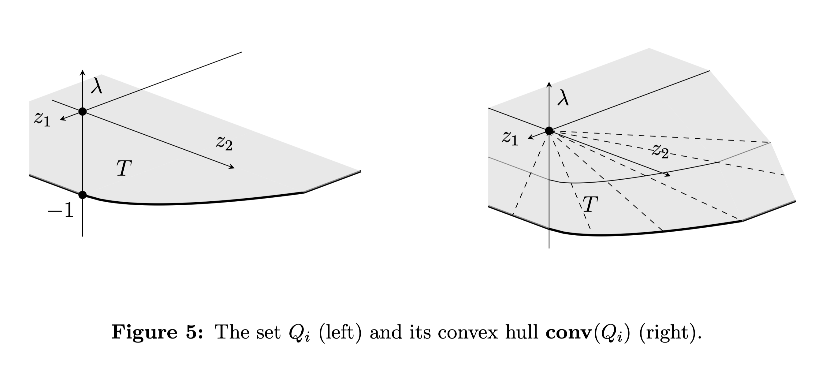
In many networks, the number of edges (the number of sets $m$ ) is much larger than the number of nodes (the net flow dimension $n$ ). Although fixed costs make this problem nonconvex, the relaxation often has an integral solution. And even when I had to round the solution to the relaxation, the difference in objective value between the relaxation solution (a lower bound) and the rounded solution (feasible, maybe not optimal) was typically well under 1%.

These types of problems sit right outside the boundary of convex optimization. Fortunately, the more nonconvex sets you have, the closer to this boundary you get.

Thank you to Logan Engstrom for helpful comments on a draft of this post.

Footnotes

[1]	Don't get me started on those that take complexity theory as gospel.

[2]	That said, many of these transformations are not obvious. I wish there were better tools to automatically search for equivalent convex problems.

[3]	The Minkowski sum of sets $A$ and $B$ is $A + B = \{a + b \mid a \in A \quad\text{and}\quad b \in B\}$ .

Proof of the lemma

This largely follows the proof in Bertsekas' Convex Optimization Theory.

Let $S = S_1 + \cdots + S_m,$ so $\mathbf{conv}(S) = \sum_{i=1}^m \mathbf{conv}(S_i)$ . Any $y \in \mathbf{conv}(S)$ is a sum of $x_i$ 's each in $\mathbf{conv}(S_i)$ . Therefore,

y = \sum_{i=1}^m x_i = \sum_{i=1}^m \sum_{j=1}^n \alpha_{ij} z_{ij},

where $z_{ij} \in S_i$ , $\alpha_{ij} \ge 0$ , and $\sum_{j=1}^n \alpha_{ij} = 1$ for each $i = 1, \dots, m$ . We can rewrite the above as

\begin{bmatrix} y \\ 1 \\ \vdots \\ 1 \end{bmatrix} = \sum_{i=1}^m \sum_{j=1}^n \alpha_{ij} \begin{bmatrix} z_{ij} \\ | \\ e_i \\ | \end{bmatrix},

where $(y, 1, \cdots, 1) \in \mathbf{R}^{n+m}$ . By Caratheodory's Theorem, we can write the left hand side as a sum of $n+m$ vectors. Since each $x_i$ is a convex combination of the $z_{ij}$ 's, we much have some $z_{ij} > 0$ for each $i = 1, \dots, m$ . There are only at most $n$ positive $z_{ij}$ 's left. Thus, at most $n$ $x_i$ 's are not in $S_i$ (and are instead in $\mathbf{conv}(S_i)$ ). (Equivalently, $z_{ij} = 1$ for $m - n$ indices)